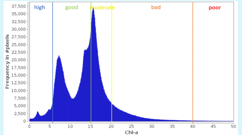
Since it is the essential pigment in phytoplankton, it can be used as a proxy for algal biomass, and as phytoplankton constitutes the base of aquatic food web, Chl-a concentration can tell us food availability, something important for example, for shellfish farmers. Furthermore, in coastal waters, phytoplankton biomass serves as an important water quality parameter since the abundance of algae can potentially indicate the degree of eutrophication in a specific water body or be related to the occurrence of Harmful Algae Blooms (HABs).
What does CoastObs offer?
CoastObs service provides highly accurate and timely geospatial information of Chl-a concentration at a spatial/temporal resolution of 300m (daily) or 10m (5 days).
How was the data validated?
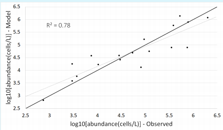
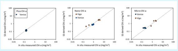
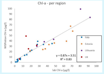
Satellite-retrieved Chl-a concentrations were validated against ground data collected close in time to the satellite overpass. The Chl-a samples collected by UVIGO, CNR, USTIR and HZ were analysed at University of Stirling using High Performance Liquid Chromatography (HPLC).
Case study example: Chlorophyl-a maps in the Galician area.
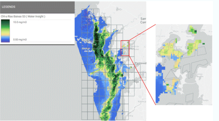
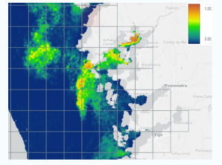
Figure 1. The map shows a scale of the chlorophyll-a present in the Galician Rias Baixas waters going from a scale of 1 mg/m3 in blue to 50 mg/m3 in green. A co-ordinate raster is shown, and after zooming in raft polygons (aquaculture areas) are shown
Limitations
- Availability depends on cloud cover
- Quality of retrieval depends on sensor characteristics, can be impacted by high suspended sediment or CDOM concentrations.
- In shallow waters, bottom visibility can interfere with the signal.
Area Covered
We can cover any coastal area you may need.
]]>Since it is the essential pigment in phytoplankton, it can be used as a proxy for algal biomass, and as phytoplankton constitutes the base of aquatic food web, Chl-a concentration can tell us food availability, something important for example, for shellfish farmers. Furthermore, in coastal waters, phytoplankton biomass serves as an important water quality parameter since the abundance of algae can potentially indicate the degree of eutrophication in a specific water body or be related to the occurrence of Harmful Algae Blooms (HABs).
What does CoastObs offer?
CoastObs service provides highly accurate and timely geospatial information of Chl-a concentration at a spatial/temporal resolution of 300m (daily) or 10m (5 days).
How was the data validated?
Satellite-retrieved Chl-a concentrations were validated against ground data collected close in time to the satellite overpass. The Chl-a samples collected by UVIGO, CNR, USTIR and HZ were analysed at University of Stirling using High Performance Liquid Chromatography (HPLC).
Case study example: Chlorophyl-a maps in the Galician area.
Figure 1. The map shows a scale of the chlorophyll-a present in the Galician Rias Baixas waters going from a scale of 1 mg/m3 in blue to 50 mg/m3 in green. A co-ordinate raster is shown, and after zooming in raft polygons (aquaculture areas) are shown
Limitations
- Availability depends on cloud cover
- Quality of retrieval depends on sensor characteristics, can be impacted by high suspended sediment or CDOM concentrations.
- In shallow waters, bottom visibility can interfere with the signal.
Area Covered
We can cover any coastal area you may need.
]]>